Optimal compounding with penalties

Cryptocurrency "dividends"? 🤔

Most people who are "in the know" of the cryptocurrency/defi world have probably heard of the various ways to earn "dividends" from their holdings. By leveraging earning protocols such as staking, lending, or by being a liquidity provider, people can just sit back and accrue tokens, increasing their portfolio's value. This is starkly different from the norm, which is to HODL until the price of their assets hits the moon.

Unlike those who strictly HODL, earners that continually invest their returns back into earning protocols benefit from the ✨magic✨ that is compound interest.

Unfortunately, since most cryptocurrency/blockchain projects are pay to play (due to gas fees), every time an earner wants to interact with an earning protocol, they need to pay a fee to do so. In short: You need to spend tokens to make tokens ...

This begs the question: How do we spend the least to make the most with respect to these earning protocols and compound interest?

Abstracting earning protocols

There are many methods to earn "dividends" from cryptocurrency; however, most fall into one of two types:

1. Auto compounding
2. Manual compounding

Auto compounding earning protocols will compound frequently and automatically, but usually do so for a percentage fee of your earnings. Manual compounding earning protocols, instead, require you to compound your own earnings, only having to pay for gas fees.

Despite both flavors, they both intend for you to follow the same steps:

1. Deposit tokens into the earning protocol
2. Wait for "dividends" to accrue
3. Receive/claim "dividends"

It might seem obvious at first just to choose the auto compounding type as it's simpler and easier, but just because it seems obvious does not mean it's the most profitable.

Instead of blindly following this procedure, let's take a closer look at both of these types of earning protocols and see if we can come up with an expression to model potential earnings. This will allow us to better understand the differences between both types and be better informed before investing in one of them.

To start, let's abstract out some overarching parameters (since most earning protocols can be modeled similarly to one another).

• $t$ - Time until each compound (in years)
• $n$ - Number of compounds per year
• $P$ - Initial balance
• $r$ - APR
• ${f_{gas}}$ - Fee per compound

Aside - We will assume, in the manual compounding case, that every time earnings are "claimed," they are automatically reinvested back into the protocol, effectively making it a compounding process.

Modeling auto compounding

Although most auto compounding earning protocols charge a fee, they have the nice added benefit of zero interaction. We can sit back and stack tokens knowing everything is managed for us. Predicting our future earnings in this category is simple as we can model future earnings with the compound interest formula (with some modifications):

As long as we take into account the percentage fee and APR, calculating future earnings is simple and direct.

Modeling manual compounding

Manual compounding earning protocols are more nuanced when calculating potential earnings than their auto counterparts (and are the primary focus of this post). Since we compound at our own schedule, we get to choose how fast or slow we want to do so. The obvious next question to ask is, "what is the best compounding schedule?" But before we get there, let's start from square one and create an expression to model earnings after compounding just once:

This is our base case where $P_{0}$ is our initial balance and $P_{1}$ is our balance after compounding. Now the obvious next question is what does this expression look like if we compound again? Compounding for a second time means we follow the same formula as before, except we substitute our second balance with our balance after the first compound. We will also assume our compounding schedule is at a constant rate, represented by time $t$ between compounds. This can be described as follows:

Now if we want to compound many times, we can define our future balance ${P_n}$ recursively as follows:

This recursive definition is great! But it would be nicer (and simpler to compute) if we had a closed form expression. Backing up to the $n = 2$ case, if we re-arrange a few of the terms, and substitute $t = \frac{1}{n}$, we can start to see a familiar formula appear:

Looking closely at the final expression, we can see that the leftmost component looks eerily like compound interest. That's because it is! And if we compare the formula for compound interest against this term we can see that there is a direct comparison that will be embedded for every positive $n$.

Now this is all well and good, but there are additional terms we aren't accounting for related to the fees that are paid each compounding. This can be expressed via the idea of iterative penalties which is the summation of fees subtracted from each compounding instance.

By subtracting the iterative penalty fees from compound interest, we get the following expression which is equivalent to our recursive definition:

Simplifying iterative penalties as a geometric series, we arrive at our final function, compound interest with iterative penalties (or $ciwip$).

With this expression we can now model the behavior of a manual compounding earning protocol with a compounding schedule of $n$. With this model, let's try to gain some insight into how they work with some visualizations. This will allow us to understand them better before we find the best schedule.

Understanding via visualization 📈

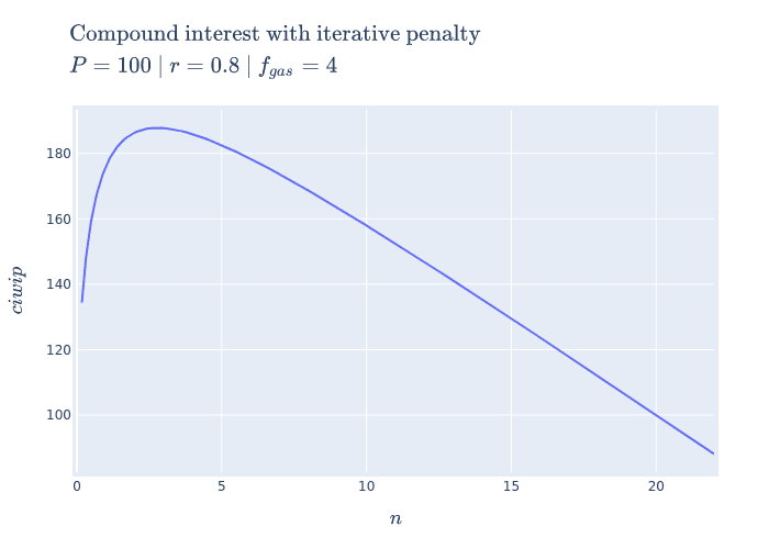
It seems most reasonable to start with a 2D plot dependent on $n$ because it's the only parameter that we can control once we put in a deposit. Holding all the other parameters constant using some arbitrary values, we get the following plot:

2D view of compound interest with iterative penalties

With this 2D view we can now get a better understanding of what optimal compounding really means.

The first intuition we can take away is that as we tend $n \rightarrow +\infty$ we see that our output value tends towards negative infinity meaning we lose more than we are gaining (which we don't want). However, there is an inflection point (around $n = 2.79$) where we make more than we lose. This means that by compounding at the right frequency, the accrued rewards are greater than the fees we need to pay to claim them.

Now we can return to our original question: "how do we spend the least to make the most?". The answer we can infer from this plot for manual compounding is "choose the optimal $n$".

Aside - Something interesting to note is that as we tend $n \rightarrow +\infty$ it looks like our function starts to become linear. We can prove this by taking the limit of the derivative of our function. We can see it's independent of $n$ meaning that even though compounding to infinity means we will keep losing, we will eventually lose at a constant rate.

$$\begin{alignedat}{2} \lim\limits_{ n \rightarrow +\infty } \frac{\partial}{\partial n}{\rm ciwip}\left(P, r, {f_{gas}}, n\right) = -\frac{{f_{gas}} e^{r} - {f_{gas}}}{r} \end{alignedat}$$

Homogenization

For the example above we used fixed parameters, but what if we changed them to be higher or lower? How would our plot change? Would we still see the same shape? To learn a little more about the shape of this function, let's unify all the parameters we can't control under some var and plot what we have left in 3D.

Doing so will give us the following expression:

Visualizing this expression gives us the following plot:

A surface 3D plot of homogenized compound interest with iterative penalties

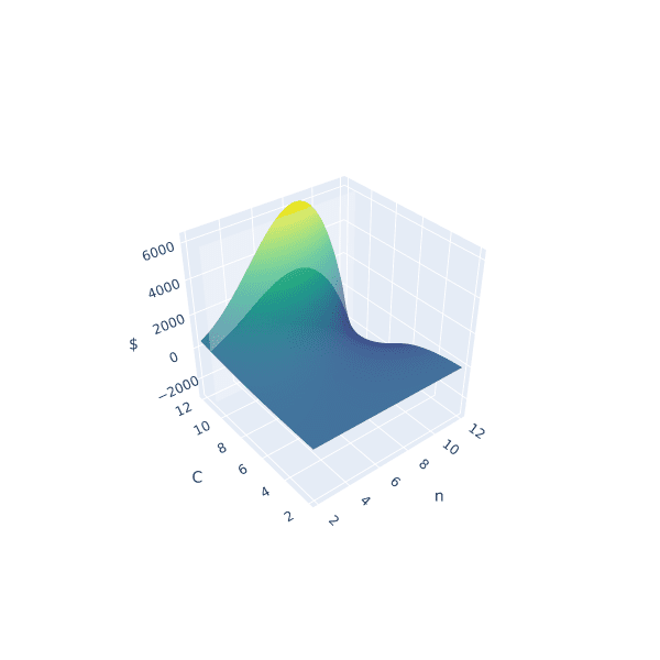
The interesting thing we can observe is that if we hold the variables we can't control constant (via $C$) and represent some choice $C$ by slicing the space with a plane (shown by the slightly opaque vertical plane), the corresponding cross section is the space of possible results of our balance as a consequence of choosing some $n$. Looking closely, there seems to be a similar shape between the intersection and the 2D plot, and if we slide the opaque plane up and down the $C$ axis, the shape seems consistent. However, this empirical observation doesn't prove anything. Instead, in search of our optimal $n$, let's explore some of the mathematical properties of our problem.

In search of optimality ⛰

We showed in the previous section that when we chose some fixed parameters for our function, there was an optimal that enables us to earn more than we lose. This is obviously an ideal case which we want to happen all the time! Unfortunately, in reality, our "fixed" parameters aren't so "fixed" and fees and APRs can change by the second. What we really want to know is: for any reasonable set of parameters, can we find the optimal number of compounds that gets us a balance greater than what we started with?

Using the gradient

One initial approach we can take is to use the gradient. If we find where the gradient is equal to zero, then we can find the extrema of our function which will allow us to find our inflection point and optimal number of compounds. Unfortunately, this isn't really tractable so we will need to find another way.

Avoiding losses

Another direction we can take is to simplify our problem by finding all the places where we lose more than we gain, and ignoring them.

We know that the space of possible compounds is from $0 \rightarrow +\infty$ and we've already established that as we compound more and more we get diminishing returns, and eventually substantial losses. To avoid these losses, we need to see where ${\rm ciwip}\left(P, r, {f_{gas}}, n\right) < P$. We can observe from our 2D graph of $ciwip$ that $P$ is intersected twice, first at $0$ and second at $n = 20.0$. Now based on what we know about this function, it makes sense that there will always be two points where ${\rm ciwip}\left(P, r, {f_{gas}}, n\right) = P$, one when we don't compound at all, and one when we are compounding too much to the point where we end up "net even." This second "net even" point is important because with it we can show that compounding beyond it will always lead to losses. To find this point we can take ${\rm ciwip}\left(P, r, {f_{gas}}, n\right) = P$, and simply solve for $n$. Doing so gets us the expression.

This means all we need to do is show that if we compound beyond this "net even" point with some positive ${\epsilon}$, we will always get less than our initial balance $P$. If we put this into an expression, we get:

And if we follow the substitution and replacement we get the expression:

This expression will always hold true as long as all the components are positive real values (which we've already established is true in the framing of our problem). This is due to the fact that the left hand component will always be negative, and the right hand component will always be positive. This means the result will always be negative.

This allows us to conclude that compounding greater than ${\epsilon} + \frac{P r}{{f_{gas}}}$ for any ${\epsilon} > 0$ we will always end up with less than our original balance.

Now we know that our optimal value must lie in between $0$ and $\frac{P r}{{f_{gas}}}$, let's try to see if we will always be able to find this optimal point.

Concavity

Now that we know our optimal value is bounded, instead of trying to find a closed form way of getting the maximum of our function, maybe we can search for it. The only problem we have now is how do we know our optimal value is easily findable? Luckily there is a property we can try to prove about our function to make finding it easier. The most ideal property we would want to prove is concavity.

If we can show that our function is concave, then we will know two important things:

1. All local maxima are global maxima
2. An optimizer will find a local maxima

In order to find out if this function is truly concave, we can leverage Jensen's inequality and check if it is true in all cases.

If we substitute our function into Jensen's inequality and supply our bounds (ignoring everything but the $n$ parameter) we get:

Substituting further and reducing we get the expression:

This final inequality will tell us if our function $ciwip$ is concave or not. It may not seem like it right away but this inequality will always be true if our components are positive real values. Let's break down this expression a bit more to see why.

First let's decompose the left hand side of our expression into two components ${\alpha}$ and ${\beta}$ as follows:

Looking at our decomposition we can first observe that ${\alpha} > 0$ because $P > P {\left| {\lambda} - 1 \right|}$.

We can also infer that ${\beta} > 0$.

Since $P {\left| {\lambda} - 1 \right|} + {f_{gas}} > P {\left| {\lambda} - 1 \right|}$, we know the base of the exponent is greater than 1. We also know that any number greater than 1 raised to a positive power will also be greater than 1. This means that ${\beta}$ must be positive.

Now that we have inferred that ${\alpha}$ and ${\beta}$ are both positive we can finally affirm that ${\alpha} {\beta} > 0$ must also be true!

Finally, since we have shown that ${\alpha} {\beta} > 0$ must be true, we have shown that Jensen's inequality must always be true, and that our function is always concave. Knowing this, and being paired with the knowledge of a bound on our search space, we can reframe our formula as an optimization problem:

In this framing, ${n^\prime}$ represents our optimal $n$ and since we know our problem is convex, we know we will always find it. Using our optimal ${n^\prime}$ allows us now to predict future earnings for $ciwip$ with the optimal compounding schedule.

Aside - You will notice that we are optimizing ${n^\prime}$ over the integers and not real values. We have to do this as there is no way we can compound a "fractional" number of times. However, we can do this and preserve concavity (from section 3.2.2 of Stephen Boyd's convex optimization book) if we say the integers are a "subset" of the reals.

Compare and contrast

Now that we have an expression to predict future earnings for optimal $ciwip$, which models manual compounding earning protocols, and an expression for auto compounding earning protocols, let's see how they compare against one another with some hand-picked parameters:

Different earning protocols modeled over time

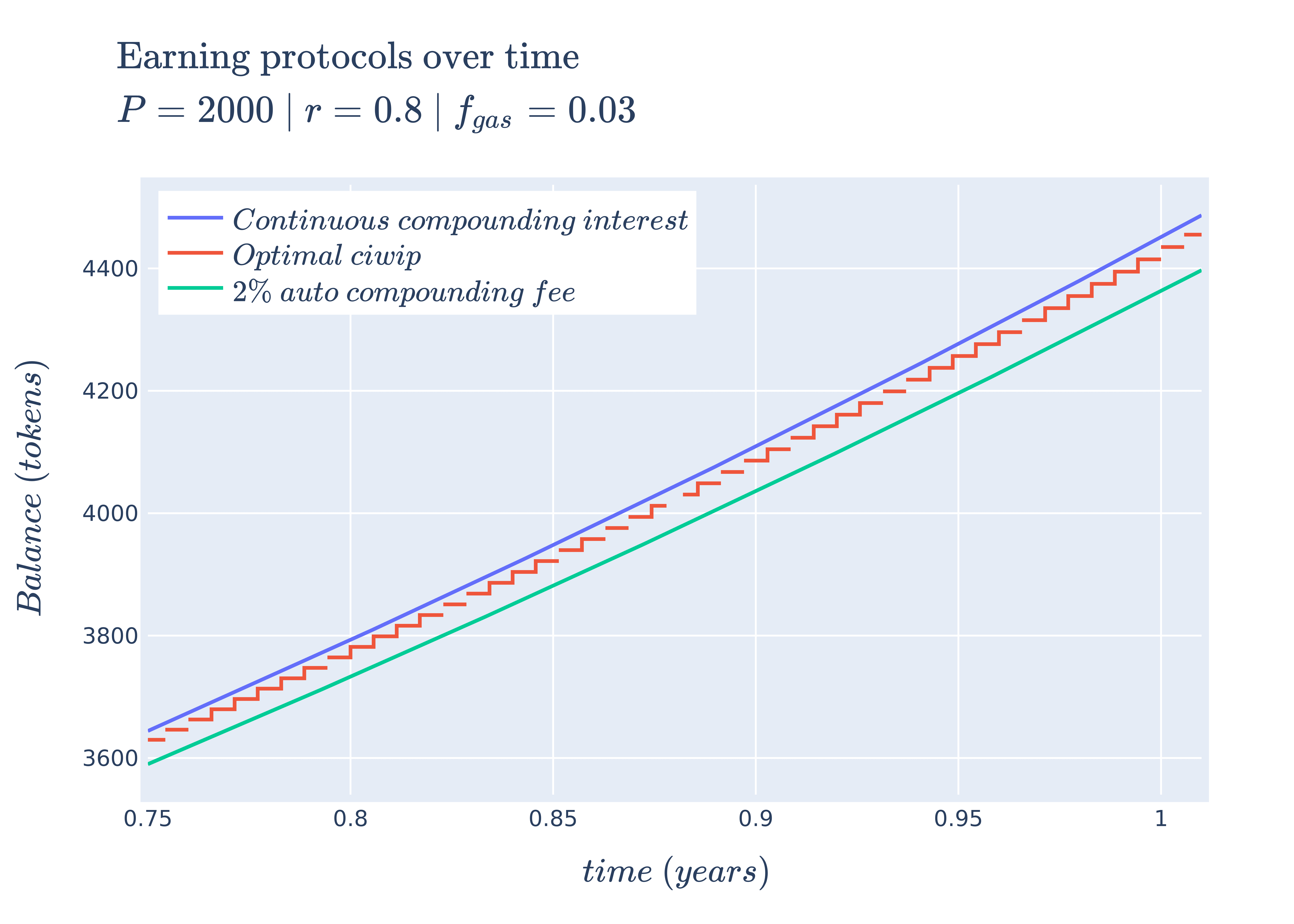
The interesting thing to take away from this plot is that given the following set of parameters, manual compounding via optimal $ciwip$ performs better than the auto compounding counterpart (with continuous compound interest performing the best). This means that if we were to assume, at the start, that auto compounding earning protocols were better and invested in them, we could be missing out on potential profits by not using optimal $ciwip$. However, if we increased the gas fee, our auto compounding variety would perform better (we will save the theory for which scenarios cause one to perform better over the other for another post).

Armed with the tools to model earnings for both compounding types, we can now make an informed decision about maximizing our profits.

Future directions

Despite the depth of this post in exploring earning protocols, we only scratched the surface as there are plenty of potentially interesting areas to explore:

1. Statistically representing earning protocol parameters:

   As mentioned earlier in this post, fees and APRs can change by the second based on a myriad of factors. If we were to represent these parameters as distributions, how would our compounding schedule or future earnings change? How could we use outside knowledge to update our hypotheses about this problem?

2. Earning protocol rebalancing strategies:

   There are many earning protocols to choose from. How should we associate risk with them? When do we leave one for another? Where do we redirect streams of earnings?

Conclusion

The world of defi and cryptocurrency continues to fascinate me as new economic experiments and protocols get launched every day. Despite the negative press, I truly believe these experiments will yield novel results and change the way we move value between one another. It also could all go to zero, but I'll enjoy the ride either way.

I hope you enjoyed and learned something new 🖐