Solving the two stocks probability puzzle

The puzzle

Last year I attended a multi lecture series "Math Explorations" at MoMath hosted by Steven Strogatz. During the final lecture, Steve showed us this interesting tweet by the creator known as @10kdiver. I encourage you to take a stab at the puzzle! Keep in mind the highlighted answer is the highest voted and not necessarily the right answer.

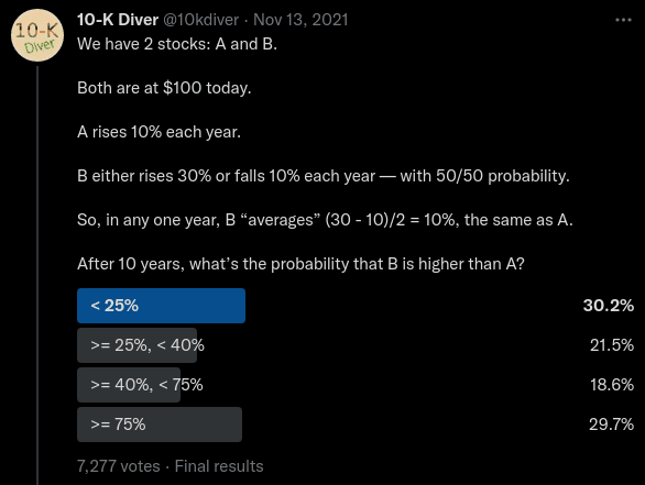
10K Divers two stocks puzzle as a tweet

The solution

Attacking this puzzle seems simple at first glance, but has an interesting non-intuitive line of probabilistic reasoning (as most probability puzzles do) that will get us the answer. In order to work towards the solution, lets start by formalize everything we know starting with stock A.

Stock A has predictable returns, meaning we can easily calculate the future price (represented as ${a_{10}}$) as follows:

It's safe to conclude that Stock A is awesome! It gets us over 2.5x our initial investment after 10 years guaranteed!

Stock B on the other hand isn't so clean cut as it's depends on how "lucky" we are and how many "wins" and "losses" occur. Without thinking about "luck" or probability, let's create an expression for stock B's future price parameterized on a single win:

For reference, $r_{n}$ represents the result of a single year (1 or 0 meaning "win" or "lose") at year $n$. $b_{n}$ represents the price of B at year $n$. But we can simplify this recursive definition of stock B's price into a singular formula based on the number of wins and losses after $10$ years.

Now that we have the tooling to calculate stock A and stock B's future price, the next step is to figure out in what scenarios does stock B overtake A. It's clear to see that after 10 years, stock B can reach multiple prices. For example, if stock B "wins" 9 years out of the 10, the future price can be calculated as:

Wawaweewa! This is almost 10x our initial investment! Albeit rare as there are only a few ways to "win" 9 times.

Stock B could also "lose" 9 years out of 10, which results in a price of:

Boooo! We lose almost half of our investment! But just like our first scenario this is also rare as there are few ways to "lose" 9 times.

The next question we should ask ourselves is how many "wins" will it take for stock B to overtake stock A? To get the answer, we can use our previous price formulation of stock B, set it equal to stock A's final price and solve for the number of "wins" it will take for B to equal A:

Simplifying and solving we get:

Now we know that after $5.46$ wins, stock B will overtake stock A. But this doesn't make sense. We don't have a way to define what a "partial" win means. To remedy this we must round up to the nearest number of wins because we are only interested in where stock B "beats" stock A.

Let's get a better understanding by visualizing this "overtake":

Figure to compare both stocks final prices

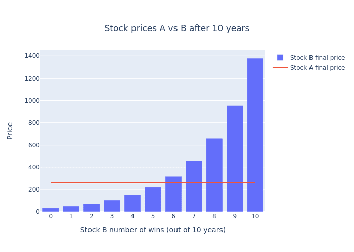
By looking at this graph we can see that stock B only starts "beating" stock A once it gets 6 wins or more.

Moving forward, knowing that we need at least 6 wins, we can now start to narrow in on our final answer by asking the next natural question, "what are the odds of winning 6 or more times". The initial urge one might say would be to perform a "sum" like so $0.5 ^ 6 + 0.5 ^ 7 + 0.5 ^ 8 + 0.5 ^ 9 + 0.5 ^ {10} = 0.03$, but this is a mistake! With this result we are instead answering the question "What is the sum of probabilities of a sequence of $6,7,8,9,10$ wins/losses?" Instead the underlying question we really want to answer is "Out of all the possible sequences of wins/losses, what is the probability of B getting 6 wins or more?"

To answer this analytically, we need to think in terms of combinatorics! Our answer will come to us if we determine the count of all winning sequences divided by all possible sequences. We can formulate this idea by using the formula "n choose k" (commonly known as the binomial coefficient formula), sum up all the ways to make $6, 7, 8, 9, 10$ wins, then divide by the number of all possible sequences of "wins" and "losses":

So $0.38$ or ">= 25%, < 40%" is our final answer!

What I find most interesting about this puzzle is that most peoples "gut" answer is no where close to the actual answer. The puzzle definitely puts into perspective the non intuitive results of calculated probabilities vs "gut" probability.

Extra credit: Stock C

Now that we solved the two stocks probability puzzle, let's extend the puzzle to make it more interesting! Call it "extra credit" 😂.

This extension was not covered by 10K Diver and is my personal contribution to the puzzle:

Along with stock A and B, we now introduce stock C.

Stock C is very similar to stock B, except alongside the possibilities of a "win" or a "lose", there is an additional equal chance of a "none" year occurring, meaning no loss or gain.

Overall Stock C has an equal chance of rising 30%, falling 10%, or staying the same.

After 10 years, what's the probability that C is higher than A?

What about C being higher than B?

Take a stab at this extension to the puzzle and continue reading for the answers.

At first one might think that we need a whole different approach to getting the solution, but we can actually just build on top of the tooling we already used to solve the original puzzle.

The first piece we need to understand is that the formula for stock C is no different than that of stock B, it's just a change of constraints.

Note: We are using $N$ instead of $n$ to indicate the number of "none" years.

If we look at the formula for the future price for stock C above, we can see that it's equivalent to stock B (because multiplying anything by 1 keeps the result the same)! However, this doesn't mean that stock C is equivalent overall to stock B. Unlike stock B, the second formula underneath is the constraint that stock C must have satisfied before calculating price.

Building on top of this new information, the next piece we need to understand is how many possible future prices can stock C reach after 10 years? We know that stock A has only 1 possible future price and stock B has 11, but what about stock C?

This can be easily calculated via combinations with replacement (aka multiset binomial coefficients). We can do this by representing stock C's final prices as unique "objects", and years be represented as "sample size" (combinatorially speaking):

We can now see that stock C has $66$ potential future prices, woweee! But how many of those future prices beat stock A?

To get a better understanding when stock C beats stock A, let's plot all the combinations of wins, losses, and nones, then color the situations where stock C beats stock A.

3d plot of outcomes of stock C that beat stock A

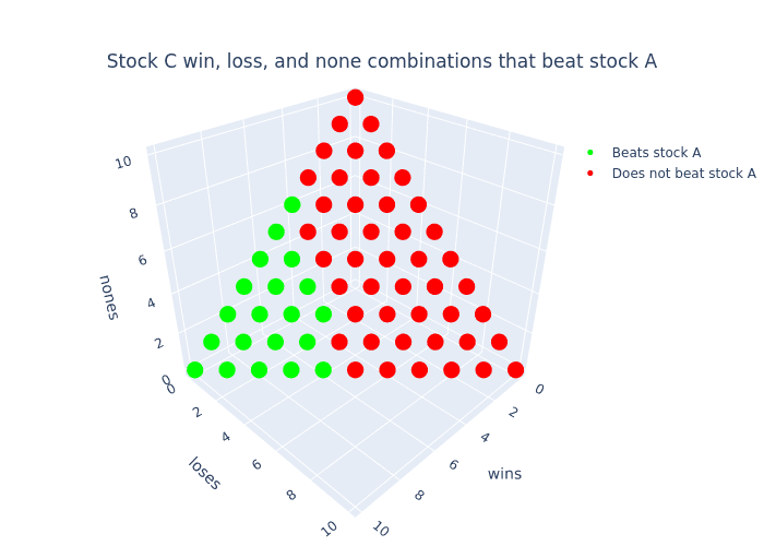
In this plot every point is a particular combination (or multiset) of "wins", "losses", and "nones" colored to indicate which final prices "beat" stock A. It's quite clear to see that there are more final prices that result in stock C losing to stock A. At this point, one might think that the answer is just the ratio between the number of dots that are green divided by the total number of dots (which is $\frac{20}{66} = 0.303$). Unfortunately this isn't the right answer. We need to remember (from the first part of this puzzle) that we need to take into account all the possible ways we can reach these final prices opposed to just looking at final prices. To count the number ways to reach these final prices, we will build on top of the previous tool we used (the binomial coefficient formula) with its natural extension: the trinomial coefficient formula 🤓📐!

With this new tool, we can now determine the number of ways stock C can beat stock A and compare that against the total number of ways stock C can reach any final price. Pulling this all together with some summations and a piecewise function we can express our final answer as follows:

This expression is pretty daunting, so let's break it down.

1. Each summation iterates across all possible "wins" and "losses" that satisfy stock C's constraint. We don't need to explicitly iterate by $N$ because we can calculate it from $w$ and $l$.
2. The denominator is summing up all the possible ways stock C can reach any of its final prices.
3. The numerator is summing up only the number ways stock C beats stock A

Performing this computation gets us a final result of $0.19$ 😮. To put this into context, that's half as much as stock B! What a terrible investment opportunity!

The interesting insight to take away here is that just because we added a new seemingly innocuous outcome (adapting stock B to stock C), doesn't mean an innocuous change in results.

Verification via Monte Carlo

So far we have done all of our probability calculations analytically (using just formulas and algebra). Another way to calculate the answers to these puzzles is to use Monte Carlo simulation!

Monte Carlo methods, or Monte Carlo experiments, are a broad class of computational algorithms that rely on repeated random sampling to obtain numerical results. The underlying concept is to use randomness to solve problems that might be deterministic in principle

-- Wikipedia

In simpler terms, the Monte Carlo methodology is used when we just want to throw a computer at a statistical problem, and get an approximate answer. So by throwing some Monte Carlo at our puzzle (via some Python / Numpy) we get the following results:

1import numpy as np
2
3stock_B = np.vectorize(
4    lambda sample: \
5    start_price * \
6    (b_perc_win ** (sample == 0).sum()) * \
7    (b_perc_lose ** (sample == 1).sum()),
8    signature="(n)->()"
9)
10stock_C = np.vectorize(
11    lambda sample: \
12    start_price * \
13    (b_perc_win ** (sample == 0).sum()) * \
14    (b_perc_lose ** (sample == 1).sum()) * \
15    (1.0 ** (sample == 2).sum()),
16    signature="(n)->()"
17)
18
19samples, years = 10_000, total_years
20stock_A_samples = (start_price * a_perc**total_years)
21stock_B_samples = np.apply_along_axis(stock_B, 1, np.random.randint(0, 2, size=[samples,years]))
22stock_C_samples = np.apply_along_axis(stock_C, 1, np.random.randint(0, 3, size=[samples,years]))
23
24print("B > A:", (stock_B_samples > stock_A_samples).mean().round(2))
25print("C > A:", (stock_C_samples > stock_A_samples).mean().round(2))
26print("C > B:", (stock_C_samples > stock_B_samples).mean().round(2))

1B > A: 0.38
2C > A: 0.19
3C > B: 0.36

And BABAM! Our Monte Carlo simulations have verified our first two answers and gave us an approximate answer for our third! See if you can find an analytical solution to the probability of stock C beating stock B!

Conclusion

Why is this puzzle worth talking about?

What makes this puzzle special is that right out of the gate you are prompted with a contradiction, namely that both stocks "average" the same. At first this is just confusing, but it's secretly a hint! The puzzle is essentially telling you "don't think in averages, try something else!"

I usually don't like puzzles that give you hints right away, but this one is an exception. It's hidden in plane sight and it's the first thing your brain gravitates too.

One of the most beautiful things I love about puzzles like these (and statistics in general) is how innately unintuitive they can be. Often times our gut instinct is starkly different than the real solution and thats OKAY! When I first saw this puzzle/tweet from Steve my first and second gut answers were wrong! Only after being given a hint from Steve to "think combinatorially" did I start to realize how to approach and solve it.

Thanks for getting this far down statistics boulevard 🎊, let me know what you think of this post in the comments below!