

The not so well known sides of cryptography
When most programmers think of cryptography, they think of things like PKI, AES, HMAC's, etc. These techniques are extremely important, but in the overall umbrella of cryptography, they are just the tip of the iceberg.
One area that doesn't get much love are polynomial commitment schemes (PCS). To change that I'm going to break down one of the most well known polynomial commitment schemes KZG10.
What is a Cryptographic Commitment?
Making a cryptographic commitment is like making a promise. It enables us to "commit" to some statement and prove later that we were abiding by it. The ones receiving the commitment can also trust that it's cryptographically hard to lie without being caught.
More formally, the two security properties that make this possible are:
- Binding: Two different statements can't make the same commitment
- Hiding: Given a commitment, nothing is known about the statement
If you want to learn more about these properties, I've written about hash based commitment schemes that goes into more detail.
Polynomial Commitment Schemes (PCS)
There are many different styles of commitments. What makes PCS unique is that instead of committing and verifying a "statement" (a.k.a just a blob of data), we are verifying a polynomial. This might not seem so special at first glance, but in PCS we get the additional utility of verifying polynomial evaluations!
In essence, this allows us to do verifiable computation on a polynomial without re-doing the evaluation ourselves.
KZG10 PCS
There are many extraordinary PCS like FRI or IPA (used in bulletproofs), but KZG10 has a few unique features compared to other schemes:
- It is pairing based
- Its proofs are constant in size (a single elliptic curve group element)
- Verification time is constant (two pairing operations)
This is awesome because when applying PCS to zero knowledge systems (like zkSNARKs), constant space and time is pretty neat! But it's not all sunshine and rainbows as the largest tradeoff of KZG10 is that it requires a trusted setup.
KZG10 as a protocol
Let's start by framing KZG10 as an example protocol. Doing so will give us a base understanding of all its components and how they fit together.
In this example protocol there will be two participants, Victoria the Verifier who wants to outsource the computation of a polynomial, and Peter the Prover who wants to evaluate the polynomial and show the evaluation is correct. We will also assume that any messages sent between them become public information.
This is a non-standard protocol, but will serve its purpose in understanding KZG10. We'll start at a high level diagram as follows:
 An example KZG10 based protocol
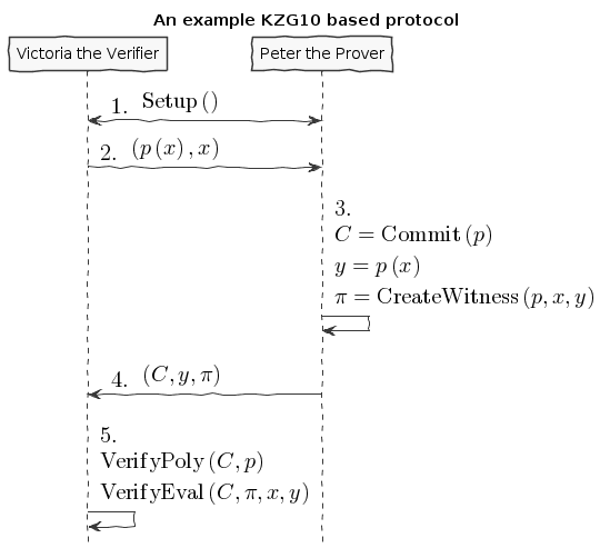
Now this is a pretty dense representation so to break it down. Here is what the variables, functions, and steps represent.
| Variable | Description |
| The desired polynomial to be evaluated of the form | |
| Point to be evaluated by | |
| Committed representation of the polynomial | |
| Proof of evaluation (not ) |
| Function | Description |
| Sets up paramaters to be used for the rest of the protocol | |
| Creates a "commitment" when given a polynomial | |
| Produces a proof of evaluation of on | |
| Checks that a commited polynomial and a polynomial coincide | |
| Checks that a committed polynomial was evaluated properly |
Steps
- Victoria the Verifier sends the polynomial with an x coordinate to be evaluated.
- Peter the Prover computes a commitment to the polynomial, the evaluation of the polynomial, and a proof of evaluation.
- Peter the Prover sends all the information to Victoria the Verifier.
- Victoria Verifier checks that Peter the Prover has evaluated the polynomial properly and has committed to the correct polynomial.
Notice that at no point will Victoria the Verifier evaluate the polynomial!
Security properties
To finish off describing this protocol, we need to address some security properties that will help thwart cheating. These properties establish a level of trust knowing that tampering and falsification will be hard:
Polynomial commitment binding and hiding:
We touched on this idea in the beginning of this post. But for this protocol, instead of applying binding and hiding to statements, we need to be sure they hold true for a polynomial.
Evaluation binding:
This property means that different evaluations of a polynomial will result in different proofs. With this we should be able to correctly identify that only proper evaluations and proper proofs will coincide in .
Correctness:
This property just means that our protocol works as expected. More formally: all commitments made by can be verified successfully by and all proofs made by can be verified successfully by .
The math behind KZG10
Now that we've explored how KZG10 works functionally, the only missing chunk left to understand is the math and cryptography behind the functions. We will mostly focus on correctness, but touch on some other security properties as well.
Trusted setups and the Common Reference String
The most important dependency that makes KZG10 work is the Common Reference String (CRS). This is just a set of public parameters agreed upon in that all participants use to compute and verify commitments and proofs. At the end of the day the CRS is just a set of elliptic curve points of the form:
What makes these points interesting is that is an unknown integer number (at least it's supposed to be).
Unlike in ECC public key cryptography where the key holder knows their private and public key ( respectively), in KZG10 we have a bunch of "public keys" with an "unknown" private key. Even though we don't know what mystical number was used to create these "public keys", we do know that each successive "public key" is defined by another successive power of .
We will use this to our advantage when we start talking about evaluating polynomials.
Why is the CRS secure?
Ensuring is a secret is very important for the security of KZG10. If we knew then we could forge commitments and proofs to our advantage (more on that later).
In order to make a CRS we could sample our own and just "not look" at what it is (which is commonly done for testing). But if many people wanted to use our sampled CRS, they would have to trust that we didn't look at 😉. In practice, cryptographers perform MPC ceremonies where many machines contribute randomness to so no one can reconstruct it without collusion. The process for generating a CRS through MPC ceremonies is a bit out of scope for this post, but these resources by Vitalik Buterin and Sean Bowe are great places to learn more.
But how do we know we can't just recover from the CRS?
We can see that, at most, breaking the CRS is as hard as ECDLP (since we can just try solving for in the second public parameter ). However the security of the CRS is usually described by the q-SDH and q-SBDH assumptions. These assumptions boil down to trying to find some number and EC points and/or . But it's been shown that an adversary has a low probability of doing so.
Polynomial commitments as elliptic curve points
In order to create a commitment for a polynomial, we need something akin to a "hash" like function to establish hiding and binding. We could just use a hash function, but we wouldn't be able to do any useful math on the output besides equality. This is where the CRS starts to become valuable. Using the CRS and some EC arithmetic, we can evaluate a polynomial on the secret number , and get an EC point out. Here's how:
Notice that evaluating our polynomial on is just the elements of the CRS multiplied by our polynomial coefficients. By progressively doing EC scalar multiplication and point addition we are effectively evaluating our polynomial on even though we don't know what is! 😲
Unfortunately we cannot commit to infinite degree polynomials. We are capped by parameters in the CRS. But is usually some wickedly high number which provides a lot of wiggle room (ex: from Zcash's powers of tau ceremony).
An important vulnerability to be aware of is that if we know , we can easily break binding by finding two polynomials that evaluate to the same point:
Luckily we can rely on the t-polyDH assumption (an extension of q-SDH) to help us establish hiding and binding and prevent this vulnerability.
Proofs of evaluation
Now that we can commit to a polynomial, the next step is to evaluate it on a known point and prove we did so by creating a proof/witness.
Aside: A "proof" and "witness" have similar definitions and are used quite interchangeably. Yehuda Lindell provides a great explanation of the distinction between the two.
The actual KZG10 paper uses the term "witness" but I believe "proof" is easier to understand.
Evaluation of a polynomial is easy, but proving we did so is not obvious. Here is the underlying math for proof creation:
Since we don't know , we must first do polynomial division between and , then evaluate the resulting polynomial with the CRS. We can also trust that there should be no remainder from this division because all terms in are of the form (this becomes important a little later).
Verifying evaluations
The proof we've just generated doesn't look like much, but it encodes a lot of useful information related to the commitment previously generated that we will use to verify its correctness.
But before we can understand how to verify evaluations, we need to talk about the primary ingredient to verification, namely pairings.
Elliptic curve pairings
Elliptic curve pairings, or "pairings" for short (defined by the operator ), are a beautiful yet extremely complicated construction. They enable us to take two points on an elliptic curve (usually in two different groups) and produce a new point in a third and different group e.g. . The main advantage of pairings are that they give us new tools to perform EC arithmetic. The primary tool we care about is the bilinear property. Bilinearity gives us the following equalities (and then some):
Understanding how pairings work is a topic for another day, but here are some resources if you're curious:
- Exploring Elliptic Curve Pairings
- BLS12-381 For The Rest Of Us
- An Introduction to Pairing-Based Cryptography
- Pairings In Cryptography
- Bilinear Pairings
- Pairings for beginners
Using bilinearity
Using this bilinear property of pairings we can now dissect and understand the underlying equality behind verifying evaluations:
Simply put, verification boils down to checking that two target group EC points are equal. By doing this simplification and rearranging of terms, we can confirm that both sides of this equality are computing the same thing. However, to better understand correctness and soundness, let's dig deeper into why this verification will fail when tampered with.
Trying to cheat verification
Let's say we want to cheat as the prover and produce a false value that will pass the test. The only way we can achieve this is by tampering with any and all of . We've already established that tampering with is hard because of binding, so instead we are left with and .
We can also clearly see that since is composed within , they must be changed together.
If we try cheating with , the naive approach is to choose our desired false value and change the term in to .
Fortunately for the verifier, this naive cheating method will most likely result in the numerator of the proof leaving a remainder when divided by . This will result in a failed reconstruction of by the verifier, and a failed equality check.
Instead we need to be smarter. To cheat without detection we need to find a such that is divisible by . Doing so will trick the verifier in the left hand pairing evaluation of resulting in a bad reconstruction of . This bad reconstruction would seem "normal" to the verifier, but actually result in a false positive.
Aside: We could try to find a equal to to cheat. But this would require us to break the q-SDH assumption.
Unfortunately for us, finding the right to cheat is not feasible. If we first observe that the terms of a correctly executed proof numerator can be simplified like so:
We see that the polynomial will always have a positive root at and will always be divisible by .
This puts us in a pickle because we can only construct polynomials of the form . Since we can only use this form, the polynomial factor theorem tells us the only polynomials we can make from that can be divided by the linear factor are the correct evaluations of ! Uh oh ... we can't cheat!
Bad for us (the cheating prover), good for the honest verifier.
Batch proofs
So far we've covered how to verify a polynomial evaluated at a single point. This is incredible by itself, but if we wanted to prove the evaluation of multiple points on a polynomial, we'd have to repeat the same protocol over and over again. This clearly isn't efficient and would result in a lot of communication and back and forth. To remedy this, we'll look at an extension of our existing KZG10 techniques and learn how to "batch" verify points on a polynomial.
To implement this, we'll build on top of the mechanisms we learned from proof creation/verification and substitute in Lagrange polynomials and zero polynomials.
What are Lagrange polynomials?
When given data, Lagrange polynomials are normal polynomials designed to interpolate or "fit" said data. It's formulation is:
What are zero polynomials?
Not to be confused with the polynomial thats just the constant "zero", a zero polynomial is a polynomial whose "zeros" (a.k.a roots) are defined by some set of data points . This can be expressed as:
Putting it together
By doing the follow substitution in with a Lagrange polynomial and zero polynomial:
And the same in :
Boom! Just like that we've added batching and have two more functions: and . But how do we know this substitution can correctly "batch" verify points?
For our "new" , if we assume all the points are legitimate evaluations of , then both and will have the same intersection points. Knowing this and performing the subtraction results in a polynomial whose roots are . This is great because our denominator (the zero polynomial) has the same roots and is therefore divisible since the product of linear factors is a factor. We can now rest assured that verification will go smoothly because since we can do a clean polynomial division in , we can also do a clean reconstruction of in by pairing with the .
The wild thing to notice is that even though we can verify many points with "batching", the size of our proof stays the same size (one EC point)! Our only limitation is the size of the CRS which determines the number of points we can verify (bounded in and ). And the size of the polynomial we can verify (bounded in ).
But we've already established that CRS's are pretty huge (sometimes ), which in practice is very practical for verifying many points and large polynomials.
Implementation
All this cryptography and math theory is great, but implementation is where the real fun begins. Luckily a KZG10 implementation depends only on elliptic curves and finite field polynomial arithmetic which most cryptography libraries include.
I choose to build off of Kryptology simply because it has a great set of cryptographic primitives where KZG10 would feel at home. You can check out my contribution here.
Moar links
PCS are just the beginning of the cryptography and zero knowledge rabbit hole. Here are some more links to learn more. Thanks for reading!

